Points on a plane
Here, we walk through the steps of building a ResNet for a simple binary classifier for points on a plane.
We train a classifier to tell two kinds of points apart, and watch the map it draws. Pick a dataset: points (x, y) on a plane, each labelled either blue dot or gold diamond. Play around with the buttons!
| find | row | x | y | label |
|---|
Training vs inference
Below is an overview of a simple, full neural network architecture.
The only difference between ResNet and a basic neural network
Inside a ResNet block
One block, opened up: the forward pass along the top row, the backward pass along the bottom row, then the update. A red box marks the two steps where a basic neural network differs.
Three kinds of thing live on that canvas:
- weights W₁, b₁, W₂, b₂: the only things that ever change, and only in the last stage.
- activations x, h, f, xout: recomputed on every forward pass.
- messages dxout, dh, dpre, dW₁, dW₂, dxin: computed on every backward pass, then consumed, the dW’s by the update and dxin by the block below.
The equations are the same at every stage and in every block; only the numbers change.
backward: dh = W₂ᵀ·dxout, dpre = dh ⊙ (1 − h²), dW₂ = dxout·hᵀ, dW₁ = dpre·xᵀ, dxin = W₁ᵀ·dpre + dxout W₁ is 8 × 2, W₂ is 2 × 8; the biases' slopes are dpre and dxout themselves. Going forward the residual block adds x back; going backward it passes dxout straight through. A basic block does neither.
Gradient descent
The update step that closed the block walkthrough above, W ← W − lr·dW, is one move: keep the guess, add a correction. Here it is with a single knob, so the whole thing fits in one picture.
Training uses the slope of the error to find where the error is smallest. One knob, w, and a bowl: the error of the line y = w·x against data that actually lies on y = 1.5·x. Start the knob in the wrong place and step against the slope.
Other iterative methods: Fixed-Point Iteration, Secant, Newton–Raphsonoptional
Descent belongs to an old family: keep the guess, add a correction sized by a slope. Three root-finders do the same thing to solve cos x = x (the equation you can solve by typing any number into a calculator and pressing cos until the display stops changing) and differ only in where the slope comes from: a fixed number (like a fixed learning rate), the last two guesses, or the true derivative.
| method | guess ← guess + correction | the correction comes from |
|---|---|---|
| Gradient descent | w ← w − lr · slope | the slope of the error; the move that trains every net on this page |
| Adam (used here) | the same, with momentum and a step size per knob | running averages of each slope and of its square, so noisy knobs take smaller steps |
| Secant | Newton, with f′ estimated from the last two guesses | no derivative needed |
| Fixed-Point Iteration | x ← g(x) | rewrite the equation as x = g(x) and keep applying g |
| Newton–Raphson | x ← x − f / f′ | the slope of f itself, to land where f = 0 |
| Residual block | x ← x + f(x) | a learned correction, applied to the data instead of to the knobs |
Non-linearity: choosing the activation function
Which one to use: whichever keeps its derivative close to 1 where the data lands. By the chain rule, the gradient that reaches the first layer is a product with one factor per layer, and each factor contains the activation's derivative σ′ at that layer. Through 50 layers that is 50 such factors multiplied together. Sigmoid's derivative never exceeds 0.25, so the product is at most 0.2550 ≈ 10−30 and the early layers stop learning: the vanishing gradient. Factors above 1 compound the other way and the gradient explodes. tanh has derivative 1 at the origin; ReLU has derivative exactly 1 for positive inputs and 0 otherwise; GELU rounds off that corner. That is the order the field moved in. ReLU is the extreme case: the identity where it is on, nothing where it is off, as close to linear as a non-linearity gets, which is the residual block's instinct too.
The maths: which bends can build any curve, and whyoptional
Six statements carry the whole argument. Each one is followed by what it means in words.
| statement | in words |
|---|---|
| layer(x) = Σⱼ w₂ⱼ · σ(w₁ⱼ·x + b₁ⱼ) | A hidden layer is a weighted sum of shifted, scaled copies of one bend σ. That is all it can ever be. |
| ∂ᵏ/∂wᵏ σ(w·x + b) at w = 0 = xᵏ · σ⁽ᵏ⁾(b) | Differentiate one copy k times with respect to its scale and the power xᵏ falls out, weighted by the bend’s k-th derivative. A derivative is a limit of differences of copies, so whenever σ⁽ᵏ⁾(b) ≠ 0 for some b, the layer can build xᵏ. |
| σ a polynomial of degree d ⇒ σ⁽ᵏ⁾ ≡ 0 for every k > d | A polynomial bend can build the powers up to xᵈ and nothing beyond: a ceiling, however wide the layer. |
| σ not a polynomial ⇒ for every k there is a b with σ⁽ᵏ⁾(b) ≠ 0 | Its Taylor series never terminates, so every power xᵏ is within reach. exp, tanh, sigmoid and sin all qualify. |
| Weierstrass: every continuous f on [a, b] is a uniform limit of polynomials | Reaching every power means reaching every polynomial, and therefore every continuous curve, as closely as you like. |
| one hidden layer is universal ⇔ σ is not a polynomial | The theorem the lines above prove (Leshno, Lin, Pinkus, Schocken, 1993). ReLU is not smooth, so the derivative step does not apply to it directly; it qualifies anyway, because sums of shifted kinks make every piecewise-linear curve, and those approximate anything. |
In one breath. A bend works when its derivatives never all die out, that is, when its Taylor series goes on forever; then copies of it can manufacture every power of x, and every power of x is enough to draw any curve. A polynomial’s series stops, so a polynomial bend caps out at its own degree no matter how many units you add. None of this says how many units are needed, or whether gradient descent will find them; that is what the line above this box is about.
A final look at training
Both networks are trained on the same points, from the same random start, with the same optimiser. Here is what each has made of the plane by its last block, the loss as training runs, and the plane after any number of blocks.
Training: the final feature space
Both nets after all 10 blocks: the points as the final straight cut sees them, and the training loss. It is the same training as the plane at the top.
Feature space after k blocks
The same journey one block at a time: the sheet folds a little more with every block. A grey mesh shows a square sheet of paper pushed through the same blocks.
Follow the trace lines: the basic neural network re-maps the whole plane at every block (x ← f(x)), so points jump and pile up; the ResNet only nudges each point a little from where it was (x ← x + f(x)), so the sheet stays a sheet.
Summary
- A network is a stack of small blocks: matrices that stretch and shear the input, a bend that folds it, and one straight cut at the end that reads off the answer.
- Training is one move, repeated: guess, measure the error, nudge every weight a little against its slope.
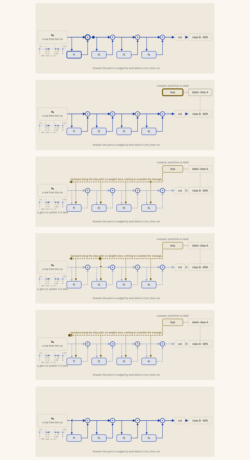
- The residual connection adds the input back at every block. A block that has learned nothing does no harm, and the correction travels back along a path with no weights on it to scramble the message. That is why deep stacks can be trained at all.
- That boundary on the plane is the whole result: a map from any point to a class, drawn by the data.
Go further
- Welch Labs, How Models Learn, a three-part series: Part 1, gradient descent · Part 2, backpropagation · Part 3, why depth works.
- Welch Labs, The most cited paper of the century is a brilliant hack: the ResNet story in twenty minutes.
- Anthropic, On the Biology of a Large Language Model.